x^3 as a non-linear unit
A wild and probably incorrect idea
UPDATE: It turns out it was not crazy at all.
These days I’m trying to learn Machine Learning(once again).
I’m more interested in understanding the fundamentals than running the race of prompt engineering and “ChatGPT” (and what is called LLM).
The other day, while watching Karpathy’s CS231n lectures, I came with a crazy idea.
So I posted something in Twitter (no Tweet without a typo).
Asking people into ML. Have anybody tested x^3 as a non-linearisation function in serious projects?
— Gonzalo Fernandez-Victorio (@gonfva) September 22, 2023
I gave a quick go to MNIST data and it seems to converge faster?
I assume we may end up with exploding gradients, but I would assume you can normalise.
What am I missing? pic.twitter.com/cno7Jo6SWH
I got no response. So I wanted to do a better write-up, and try to circulate it properly.
If somebody points me to my error, I will gladly update this post.
Quick intro to Machine learning and a bit of Linear Algebra#
At its very core, Machine Learning has a lot of Linear Algebra. A typical layer would be a linear transformation in the form of
y=W·x+b
where x is the input data (like a table) and y the output data. W and b are a group of parameters that are initially random and through “learning” (wink, wink, Machine Learning) they are modified a little bit every time until the output they produce is similar to the output we expect from them to produce.
With this process we’re doing a linear transformation (change of dimensions, rotation, translation).
Is all “machine learning” just a bunch of linear transformations?
No.
A set of linear transformations is also a linear transformation. So it wouldn’t matter how many of those layers we pile up. We couldn’t represent what we want.
The solution is that, after each one of these linear transformation, we introduce a process that is no linear. Something that “messes things up”. It introduces non-linearity, and the process is able to learn more complicated things.
These non-linear functions are also called activation functions (similar to how a neuron in Biology activates)
Non-linear activation functions#
Of those non-linear functions, the sigmoid function was used a lot in the beginning.
Sigmoid is the name for
y=1/(1+e^-x)
It is a bit expensive to compute (it doesn’t matter A LOT, but it matters). More importantly, sigmoid has a very reduced domain where sigmoid provides useful values. Outside that domain, it basically gives 0 or 1. That kills the learning process (more properly it kills the “gradient back-propagation”). In addition to that, it is not zero-centered (which means there is a bit of zig-zag on the learning).
After sigmoid, the next function to gain presence, was
y=tanh(x)
thanks to a paper in 1991 by LeCun (for the youngsters, now the AI boss in Facebook but ultimately a legend). The hyperbolic tangent works better than sigmoid. It is zero centered, but it still squashes (reduced domain with interesting values, range reduced to -1 to 1). It was used a lot until the next function appeared.
Tanh was used for a while until the function everybody uses these days came. It is called ReLU or Rectified Linear Unit. ReLU can be defined as
y=max(0,x)
So if the input value is negative, ReLU outputs 0, but if the input value is positive, it outputs the value.
Here you can see a diagram with the three functions.
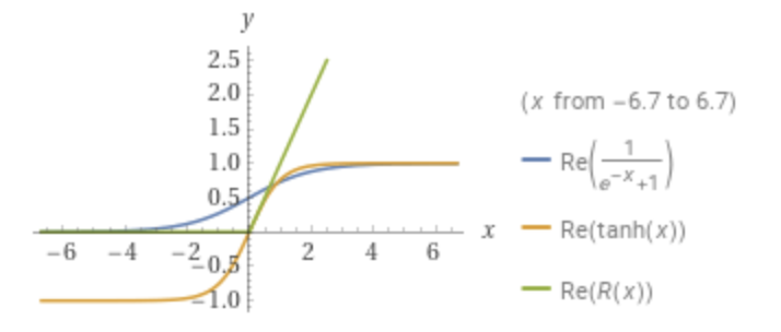 Sigmoid, tanh(x), ReLU from Wolfram Alpha.
ReLU works surprisingly well for such a simple function. It gets computed fast, it doesn’t saturate in the positive domain and it converges much faster than the other two.
However, as with sigmoid, ReLU is non-zero centered, and it also kills part of the learning process (negative gradients)
Are those the only options?#
There are other options for non-linearity.
But as I was watching the linked video, there was one obvious function that I was surprised not to see mentioned.
It is y=x3.
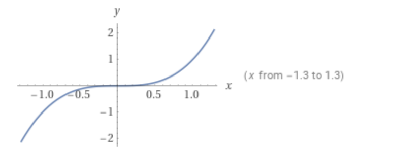 y=x3 from Wolfram Alpha.
y=x3 (also y=x^3 or cubic) is a non-linear continuous function, derivable across the domain, zero-centered, and it doesn’t saturate across the whole domain (not only in the positive region as with ReLU).
I would assume it is relatively easy to compute. Obviously ReLU is simpler to compute (ReLU is a “non-linear y=x”). But to me y=x3 is simpler than tanh.
There is one obvious problem looking at the graph. It explodes the input (the learned gradient).
I wasn’t particularly worried about that since you can do some normalization.
Now that I’m writing this, I’m more worried about the central region of the domain. We’re squashing the gradient for small values. But I perceive the learning could escape that region easily.
And I didn’t think about the central region at the time.
I just … tested it.
Time to fire up Jupyter#
So I went to Jupyter Notebook (sort of a Microsoft Word for Machine Learning :D) and opened my playground with my favorite machine learning problem.
It is based on MNIST, which is a set of pictures of hand-written numbers, and a label for each picture (sort of “the real truth”).
For example, we have a picture like the following and a label of 6
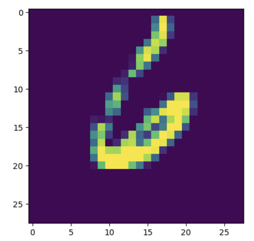 Is it a 6? From MNIST.
You train your model using the MNIST training data and then you test your model using testing data (a different portion of MNIST data)
I built a simple model (basically a one hidden layer loosely based on a book I’m reading and I highly recommend).
You can find the code below so that people can copy and paste from here.
# Lets load the data
from tensorflow.keras.datasets import mnist

(train_images, train_labels), (test_images, test_labels) = mnist.load_data()

# Now let's prepare the data into single vectors of between 0 and 1
train_images_input = train_images.reshape((60000, 28*28)).astype("float32")/255
test_images_input = test_images.reshape((10000, 28*28)).astype("float32")/255

# Now let's prepare the model
from tensorflow import keras
from tensorflow.keras import layers
import tensorflow as tf

#Set a specific seed so that things are reproducible
keras.utils.set_random_seed(1972)

#First the model with relu as an activation
print("Relu as activation model\n\n")

model_relu = keras.Sequential([
    layers.Dense(100, activation = 'relu'),
    layers.Dense(10, activation = 'softmax'),
])

model_relu.compile(optimizer = 'rmsprop',
              loss = 'sparse_categorical_crossentropy',
              metrics = ['accuracy'])

history_relu=model_relu.fit(train_images_input, train_labels, epochs=10, batch_size=128)

#Then the model with y=x^3 as activation
print("\n\ny=x^3 as activation model\n\n")

@tf.function
def cubic(x):
  return (tf.math.pow(x, 3))


model_cubic = keras.Sequential([
    layers.Dense(100, activation = cubic),
    layers.Dense(10, activation = 'softmax'),
])

model_cubic.compile(optimizer = 'rmsprop',
              loss = 'sparse_categorical_crossentropy',
              metrics = ['accuracy'])

history_cubic=model_cubic.fit(train_images_input, train_labels, epochs=10, batch_size=128)


# We test both models
test_relu = model_relu.evaluate(test_images_input, test_labels)
test_cubic = model_cubic.evaluate(test_images_input, test_labels)


print("Test relu", test_relu)
print("Test cubic", test_cubic)

loss_relu = history_relu.history["loss"]
loss_cubic = history_cubic.history["loss"]
epochs = range(1, len(loss_relu) +1)

plt.plot(epochs, loss_relu, "b", label="Training loss for ReLU")
plt.plot(epochs, loss_cubic, "r", label="Training loss for x^3")

plt.title("Training and validation loss per epoch")
plt.xlabel("Epochs")
plt.ylabel("Loss")
plt.legend()
plt.show()
Local results#
Before showing my results, I need to stress that there is an issue on my local environment (I will explain why later).
When I tested on my local environment (iMac 2027 with Radeon 580 and the metal plugin to use the GPU), I got were the following
Test relu [0.29031872749328613, 0.9222999811172485]
Test cubic [0.1919427067041397, 0.9718999862670898]
92.2% test accuracy with ReLU compared to 97.2% test accuracy with x^3.
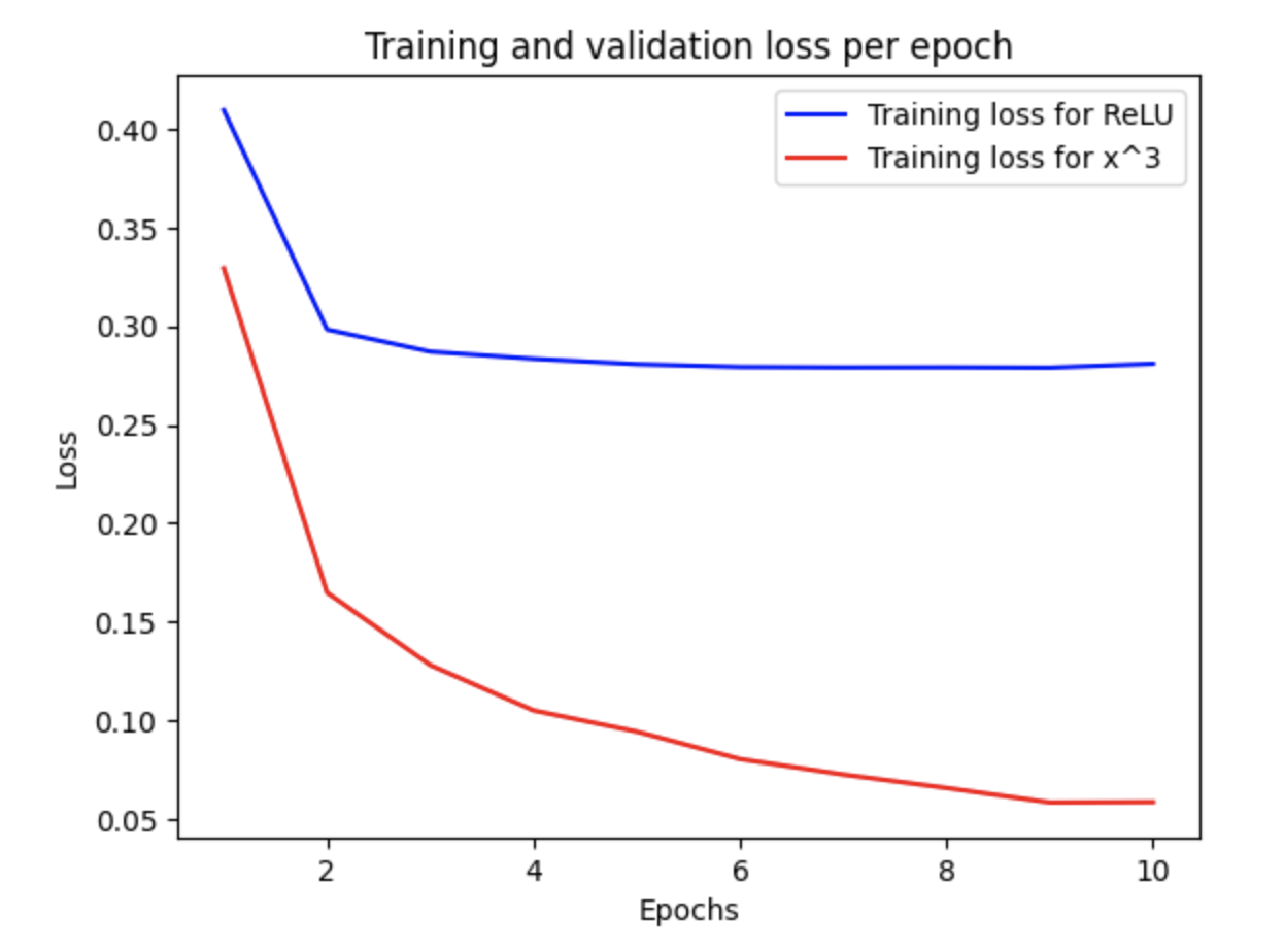 Loss per epoch, local environment.
Seeing the loss per epoch was like “this is surreal”.
Faster.
Better.
“What did I just do?”
Colab#
Then I went to colab. Colab is a way to execute a Jupyter Notebook online (for free!!). No need for a GPU, nor installing packages.
It is a service provided by Google. You only need a Google account.
I used the same code as in my local environment (here you can find the notebook)
Test relu [0.07596585899591446, 0.9776999950408936]
Test cubic [0.21662236750125885, 0.9711999893188477]
97.8% test accuracy with ReLU vs 97.1% test accuracy with x^3.
Meh.
The plot for the Loss, is also unimpressive.
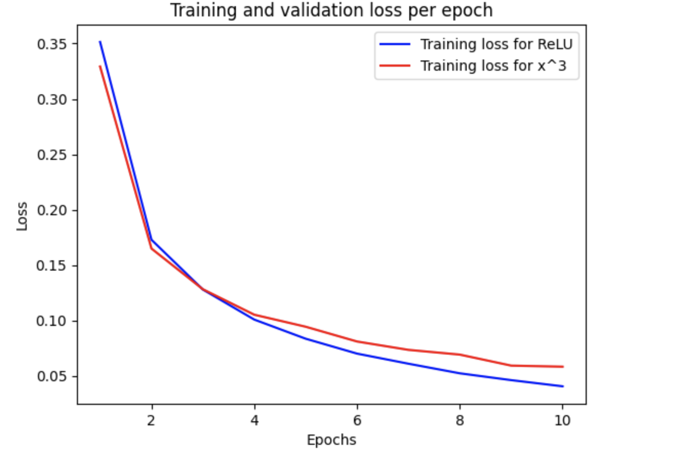 Loss per epoch, colab environment.
But in any case, even with the results in Colab, you can see y=x3 doesn’t behave bad. ReLU works better in this specific instance (and environment), but y=x3 is close.
Why nobody (to my knowledge) uses it?
Is it just because ReLU is good enough?
Local vs colab#
I still don’t know why the discrepancy from my local environment. Both have the same seed. Both use Tensorflow 2.13.0. The underlying hardware is different, but I would assume the results would be more deterministic. sIs it because I’m using the metal plugin on my Mac? I don’t know.
It seems the issue is a bug in the metal plugin
Previous work#
I did a quick search on papers, and I couldn’t find anything.
I asked ChatGPT and it told me of course y=x3 has been used as an activation function, but when pushed, showed nothing
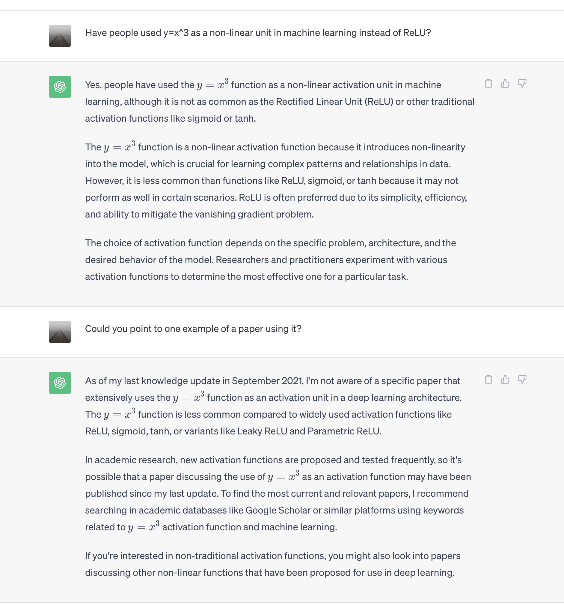 ChatGPT hand-waving.
I also asked Bard with similar explanation.
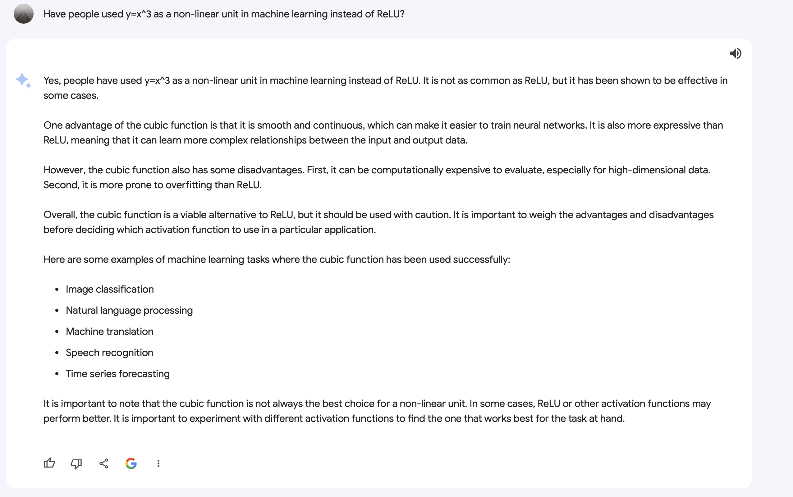 Bard hand-waving.
When pushed, it gladly produced a (fictitious?) paper.
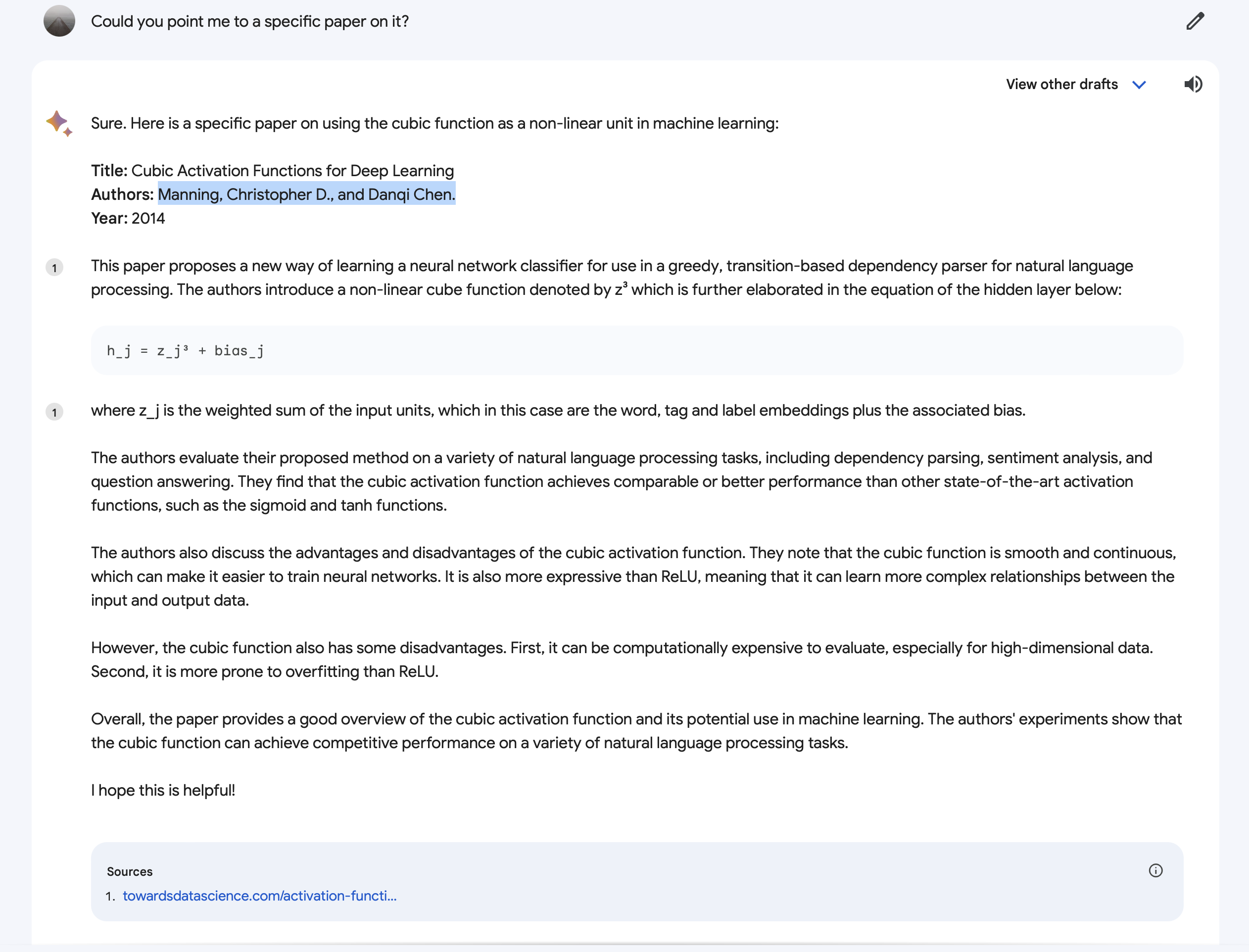 Too much LSD, Bard.
Title: Cubic Activation Functions for Deep Learning
Authors: Manning, Christopher D., and Danqi Chen.
Year: 2014
I invite you to find a paper “Cubic Activation Functions for Deep Learning” by Manning and Chen in 2014. I couldn’t.
However, the link at the bottom of Bard’s response does exist.
If you visit that page, at the end, there is a mention to y=x3 and an investigation with the title “A Fast and Accurate Dependency Parser using Neural Networks”.
The link that appears on the “Towards data science” page doesn’t work.
But searching for “A Fast and Accurate Dependency Parser using Neural Networks” did provide results.
Here, you have a proper link
https://aclanthology.org/D14-1082.pdf
And a quote
In short, cube outperforms all other activation functions significantly and identity works the worst. Concretely, cube can achieve 0.8% ∼ 1.2% improvement in UAS over tanh and other functions, thus verifying the effectiveness of the cube activation function empirically.
I was not crazy!!!
Conclusion#
Is y=x3 as a non-linearity such a crazy idea? Has anybody tested it for serious work? Has anybody tested other similar non-liberalities (y=x3+x comes to mind)? Is this worth exploring further?
So it turns out some people have tried to use y=x3 before.
It was an exhilarating moment to think you have discover something truly remarkable.
But it is good to know you are not crazy. Simply you are not the first.
Still intrigued why y=x3 is not more widely used.